使用scikit-learn和Keras建立房价估价模型

之前曾写过一篇抓取 搜房网 (fang.com) 房源数据并用 tflean 搭建神经网络进行房价分类的文章。

本文算是上面这篇文章的第二个版本：使用 scikit-learn 和 Keras 来对广州二手房房源数据搭建 回归模型 进行房源价格的估价。

数据抓取

相比于第一次抓取时，搜房网对房源页面进行了改版，因此之前所使用的抓取脚本不能使用了。于是又用 beautifulsoup 改了一遍，解析取出每一项信息然后结构化。

然后再对各项非数字内容进行数字映射，如：

regions = {'天河': '1.0', '荔湾': '2.0', '海珠': '3.0', '越秀': '4.0', '白云': '5.0', '番禺': '6.0', '黄埔': '7.0', '增城': '8.0', '花都': '9.0', '从化': '10.0', '南沙': '11.0'}  

最终的部分结果如下：

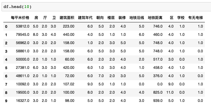
需要说明的是，我排除了每平米价格在 20万 以上的房源 ( 只有 3 例 )，土豪的世界我并不关心。

跟上一次抓取数据时相比，搜房网目前还能抓到房源是否在哪条地铁线路附近、距离地铁多远。

常识告诉我们，这也是影响房价的一个重要因素，因此也作为了特征值。

数据总行数为 10309 ：

In [4]: df.shape[0]  
Out[4]: 10309  

先看下两个图了解下房价数据：

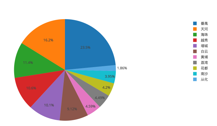
( 广州各区房源比例 )

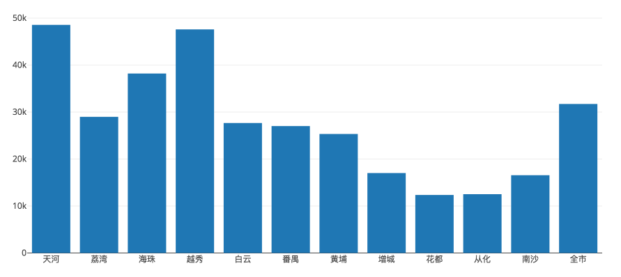
( 广州各区平均房价，最后一列为全市均价 )

具体均价如下：

{
    '天河': 48545.516516516516,
     '荔湾': 28983.626349892009,
     '海珠': 38201.262574595057,
     '越秀': 47588.640838650863,
     '白云': 27656.089361702128,
     '番禺': 27007.389256198348,
     '黄埔': 25335.879492600423,
     '增城': 17014.85277246654,
     '花都': 12356.367205542725,
     '从化': 12507.666666666666,
     '南沙': 16559.167076167076,
     '全市': 31709.176156756232
 }

上一次抓数据的时候(四月份)，全市均价还是 28995.8 ，三个月内广州的房价又上涨了 2713.4 元每平米。

备注：数据收集日期：2017/07/23 - 2017/07/25

导入数据并分为训练数据和测试数据

from pandas import read_csv  
df = read_csv('./dataset.csv')

train_ = df[0:df.shape[0]-1000]  
test_ = df[df.shape[0]-1000:]

predictors = ['房','厅','卫','建筑面积','建筑年代','朝向','楼层','装修','地铁沿线','地铁距离','区','学校','有无电梯']  
X_train = train_[predictors]  
y_train = train_['每平米价格']  
X_test = test_[predictors]  
y_test = test_['每平米价格']  

将最后 1000 条数据作为验证模型正确率而使用的测试数据，其余数据为训练数据。

选择 SVR 模型

使用 scikit-learn 的 SVR() 模型，使用默认的核函数 rbf

class sklearn.svm.SVR(kernel='rbf', degree=3, gamma='auto', coef0=0.0, tol=0.001, C=1.0, epsilon=0.1, shrinking=True, cache_size=200, verbose=False, max_iter=-1)  

gamma 默认值为 1/n，其中 n 为特征值的数量，我们的例子中 n = 13，折中取了 0.1。

另外一个比较重要的参数是 C (惩罚因子，即对误差的宽容度。C 越高，说明越不能容忍出现误差，容易过拟合。C 越小，容易欠拟合)。

具体原理可以参考这篇文章

先简单测试下 C 参数：

from sklearn.svm import SVR

for i in range(0, 7):  
    C = 10**i
    clf = SVR(kernel='rbf', C=C, gamma=0.1)
    clf.fit(X_train, y_train)
    print "C=%d, score=%f" % (C, clf.score(X_train, y_train))

输出如下：

C=1, score=-0.031758  
C=10, score=-0.020476  
C=100, score=0.061383  
C=1000, score=0.295201  
C=10000, score=0.765092  
C=100000, score=0.995138  
C=1000000, score=0.999077  

结果也验证了 C 越大，对于训练集的数据的准确度越高，先选择 C=1000000，至于是否会过拟合，我们等下再用测试集数据来验证下情况。

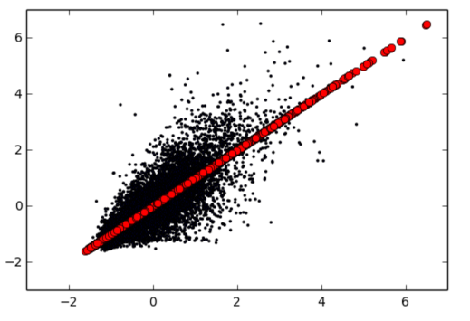
训练结果

import matplotlib.pyplot as plt

clf = SVR(kernel='rbf', C=1000000, gamma=0.1)  
clf.fit(X_train, y_train)

print clf.score(X_train, y_train)

predict = clf.predict(X_train)  
plt.scatter(predict, y_train, s=2)  
predict_y = clf.predict(X_train.values[4])  
print "predict: %.2f, actually: %.2f" % (predict_y, y_train.values[4])  
plt.plot(predict_y, predict_y, 'ro')  
plt.plot([y_train.min(), y_train.max()], [y_train.min(), y_train.max()], 'k--', lw=2)  

输出结果：

0.999076822472  
predict: 49999.90, actually: 50000.00  

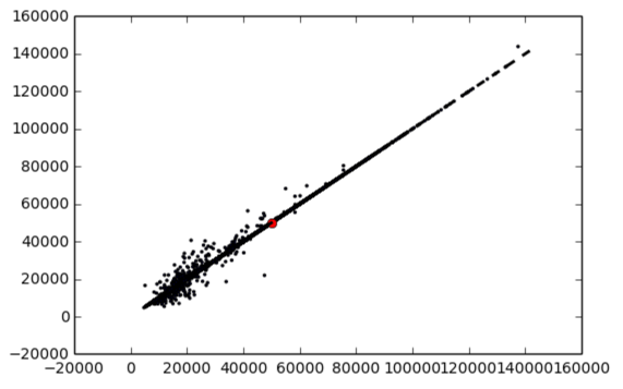
斜线为真实值线，黑点为预测值，从图上可以看到这个模型在训练集上的预测值和真实值基本吻合了。

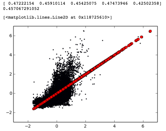
使用测试数据验证模型准确度

predict_test = clf.predict(X_test)  
print clf.score(X_test, y_test)  
plt.scatter(predict_test, y_test, s=2)  
plt.plot([y_test.min(), y_test.max()], [y_test.min(), y_test.max()], 'k--', lw=2)  

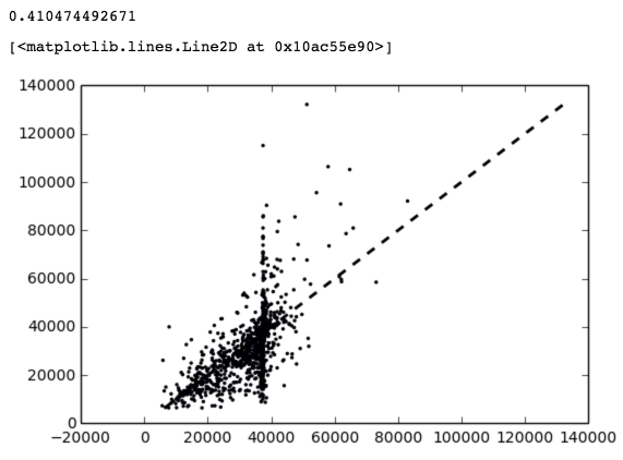
可以看到数据比较明显地分为了两拨，一拨是比较拟合真实值的斜线，另外一拨是在 x=40000 附近的垂直线。( 不明白为什么会出现这种集中在某个预测值的情况 )

准确率只有 41% ，再用 sklearn 的交叉验证函数跑 10 遍：

from sklearn.model_selection import cross_val_score

y = df['每平米价格']  
X = df[predictors]  
scores = cross_val_score(clf, X, y, cv=10)  
print scores  
print scores.mean()  

cross_val_score 函数会自动将全部数据分为 10 份，然后将其中 9 份数据作为训练集，剩下的一份作为测试集，然后会跑 10 次交叉验证。

( 跑了好久 ... )

输出结果：

[ 0.37906349  0.3947758   0.5191052   0.44455579  0.45646649  0.39464724
  0.4439831   0.4434501   0.41471762  0.39988068]
0.429064549048  

可以看到平均下来的准确度也就 42.9% 。

优化模型

改下惩罚因子试下是否有改善：

clf = SVR(kernel='rbf', C=50000, gamma=0.1)  
clf.fit(X_train, y_train)  
print clf.score(X_train, y_train)  
scores = cross_val_score(clf, X, y, cv=10)  
print scores  
print scores.mean()  

( 又跑了好久 ... )

结果：

0.985096477399  
[ 0.37902499  0.40034578  0.52363507  0.44748625  0.44871473  0.39534226
  0.43854683  0.4470296   0.41939679  0.40100924]
0.43005315467  

嗯，提高了 0.1%。

做下 Grid Search，意思是给出备选参数值，让它自动跑出一个最佳的参数值：

from sklearn.model_selection import GridSearchCV  
parameters = {'C': range(30000, 100000, 10000)}  
svr = SVR(kernel='rbf', gamma=0.1)  
clf = GridSearchCV(svr, parameters, cv=10)  
clf.fit(X, y)  
print clf.best_params_  

( 又跑了好久 ... )

结果：

{'C': 70000}

用 C=70000 重新跑了一次交叉验证：

结果：

[ 0.38117769  0.39773934  0.52183782  0.44646927  0.45482664  0.39650662
  0.44513795  0.44663406  0.41807075  0.4017944 ]
0.431019453481  

又提高了 0.1% ...

看下 scikit-learn 的文档，其中有提到 数据预处理 方面的问题：

个人理解，不太准确，大概的意思是将每个特征值按一定的规则缩放到一个比较小的范围。好比说从 1 到 100，误差可能会较大，但是缩放到从 0 到 1 的范围，误差就相对较小。

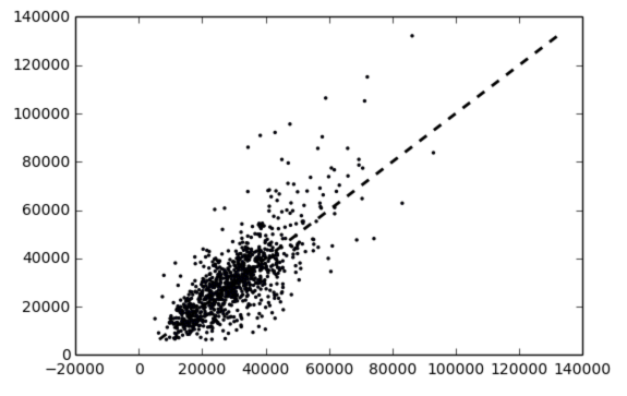
预处理之后的模型情况如下：

from sklearn import preprocessing

X = preprocessing.scale(X_train)  
y = y_train  
clf = SVR(kernel='rbf', C=40000, gamma=0.1)  
clf.fit(X, y)  
print "training score: %f" % clf.score(X, y)

X_test = preprocessing.scale(X_test)  
predict_test = clf.predict(X_test)  
print "testing  score: %f" % clf.score(X_test, y_test)  

( 需要注意的是，必须对训练数据和测试数据都进行 scale 操作；之前已做了 Grid Search，scale 之后的训练数据，最佳的 C 参数为 40000 )

结果：

training score: 0.712182291727  
testing  score: 0.575817605735  

可以看到虽然训练集的表现不甚理想，但是测试集的准确度比之前上升了 13% ，达到了 57.6%，看起来效果还是不错的。

对数据做了 scale 之后有一个问题，比如说我有一个新的数据需要预测，这时候我根本不知道应该怎么缩放以适应训练好的模型，所以需要记录下缩放的规则，然后用规则对新数据做同样的 scale 变换，才能进行预测：

scaler = preprocessing.StandardScaler().fit(X_train)  
new_data = [3.0,2.0,1.0,84.0,8.0,6.0,2.0,4.0,3.0,200.0,1.0,1.0,1.0]  
new_data = scaler.transform(new_data)  
print clf.predict(new_data)  

接下来，我们再用所有数据做下交叉验证，看下准确率：

y = df['每平米价格']  
X = preprocessing.scale(df[predictors])

scores = cross_val_score(clf, X, y, cv=10)  
print scores  
print scores.mean()  

结果：

[ 0.55006725  0.54573057  0.61465035  0.52750594  0.59165464  0.57390134
  0.6096038   0.55271578  0.50174115  0.57151666]
0.563908747408  

预测值如下，可以看到不像之前那样分为两拨了：

之后再做了 C 和 gamma 两两组合的 Grid Search，并没有得到比较明显的提升。

Give me more data!

再次收集了近 3000 条数据 (共 12937 条数据)，再次按照之前的步骤进行参数选择，重新执行交叉验证，可以看到准确度进一步提升了 2%：

[ 0.58394156  0.57893039  0.61247822  0.54683733  0.59447176  0.62030941
  0.6107769   0.5726037   0.56656728  0.55000072]
0.583691726816  

嗯，考试前多做点习题还是很有用的。

特征选择

特征选择本来应该在训练模型之前进行。特征选择的作用在于分析出影响最大的几个特征值，排除一些次要的特征值，可以提高训练的速度，但是对于准确度来说，可能会提高也可能会降低，说不定。

不过我们在这里做下特征选择，看下影响房价的最重要的五个因素是什么：

from sklearn.feature_selection import RFE  
model = SVR(kernel='linear')  
rfe = RFE(model, 5)  
rfe = rfe.fit(X.values, y.values)  
for i, v in enumerate(rfe.support_):  
    if v:
        print predictors[i]

结果如下：

房
卫
地铁沿线
区
学校

( 说明下，上面的五个特征值的重要性并不是排序的 )

上面说明了这么个结论：在哪个区、是否在地铁附近、有无学位、房间数和卫生间数 是影响房价的最重要的五个因素。

貌似也符合常识。

模型的保存和导入

训练好的模型应当保存下来，方便导入。

from sklearn.externals import joblib  
joblib.dump(clf, './model.pkl')  

导入：

clf = joblib.load('./model.pkl')  

深度学习

接下来尝试用深度学习做回归。

这里使用 Keras 的 scikit-learn 接口包装器 ( keras.wrappers.scikit_learn.KerasRegressor ) 来进行房价的回归估值。

需要导入的模块：

from pandas import read_csv  
import numpy  
from keras.models import Sequential  
from keras.layers import Dense  
from keras.wrappers.scikit_learn import KerasRegressor  
from sklearn import preprocessing  
from sklearn.pipeline import Pipeline  
from sklearn.model_selection import KFold  
from sklearn.model_selection import cross_val_score  
from sklearn.cross_validation import cross_val_predict  
import matplotlib.pyplot as plt  

导入数据、划分训练集和测试集，与之前用 scikit-learn 一样：

train_ = df[0:df.shape[0]-1000]  
test_ = df[df.shape[0]-1000:]

predictors = ['房','厅','卫','建筑面积','建筑年代','朝向','楼层','装修','地铁沿线','地铁距离','区','学校','有无电梯']

y_train = train_['每平米价格']  
X_train = train_[predictors]  
X_test = test_[predictors]  
y_test = test_['每平米价格']  

scale 预处理：

X = preprocessing.scale(X_train)  
y = preprocessing.scale(y_train)

x_scaler = preprocessing.StandardScaler().fit(X_train)  
y_scaler = preprocessing.StandardScaler().fit(y_train)  

( 在使用 SVR 时，我没有做 y 的 scale 操作，因为发现把 y 数据 scale 之后，模型训练了一晚上都没有出结果，不知道是什么原因。)

建立模型：

def nn_model():  
    model = Sequential()
    model.add(Dense(13, input_dim=13, kernel_initializer='normal', activation='relu'))
    model.add(Dense(6, kernel_initializer='normal', activation='linear'))
    model.add(Dense(1, kernel_initializer='normal'))
    model.compile(loss='mae', optimizer='rmsprop')
    return model

Dense 是全连接层，第一层全连接层，我们的数据有 13 个特征值，所以 input_dim 参数为 13。

activation 为激励函数，第一层这里选择了 relu。

然后再加一层全连接层作为隐藏层，激励函数选择 linear，参考这个链接：链接1

损失函数只能选择 mse 或者 mae，我这里用了 mae。

优化器用 rmsprop，当然也可以用 adam 之类的。

接下来使用 KFold 来做交叉验证，参考这个链接：链接2

seed = 7  
numpy.random.seed(seed)  
estimators = []  
estimators.append(('mlp', KerasRegressor(build_fn=nn_model, epochs=200, batch_size=32, verbose=0)))  
pipeline = Pipeline(estimators)  
kfold = KFold(n_splits=5, random_state=seed)  

开始交叉验证：

scores = cross_val_score(pipeline, X, y, cv=kfold)  
print scores  
print scores.mean()

plt.scatter(predicted, y, s=2)  
plt.plot(y, y, 'ro', lw=2)  

结果如下：

需要注意的是，这里的 score 并不像用 scikit-learn 的 SVR 时的准确率，而是 loss 函数的数值，即 mae ( Mean Absolute Error )，因为 accuracy 是不能参考的。参考链接1：

从打印的预测值点图来看，比较发散，并不算理想。

我们尝试改进一下模型，加多一层隐藏层：

def nn_model():  
    model = Sequential()
    model.add(Dense(13, input_dim=13, kernel_initializer='normal', activation='relu'))
    model.add(Dense(6, kernel_initializer='normal', activation='relu'))
    model.add(Dense(3, kernel_initializer='normal', activation='linear'))
    model.add(Dense(1, kernel_initializer='normal'))
    model.compile(loss='mae', optimizer='rmsprop')
    return model

然后将训练轮次增加到 500：

estimators.append(('mlp', KerasRegressor(build_fn=nn_model, epochs=500, batch_size=32, verbose=0)))  

结果：

[ 0.42803601  0.39274284  0.41864015  0.40990664  0.38228733]
0.406322592681  

可以看到 mae 减少了 11%，意味着模型的预测值更加准确了，而预测值点图也说明了这点：

用一个自制的检查准确度的函数来看下，假设预测值与实际值误差不超过 10% 为准确的话：

import math

X_test = test_[predictors]  
y_test = test_['每平米价格']

total = len(y_test)

cnt = 0  
X_test = preprocessing.scale(X_test)  
predicted = model.predict(X_test)  
for i,v in enumerate(predicted):  
    p = y_scaler.inverse_transform(v)
    r = y_test.values[i]
    if math.fabs(r - p)/r < 0.1:
        cnt += 1
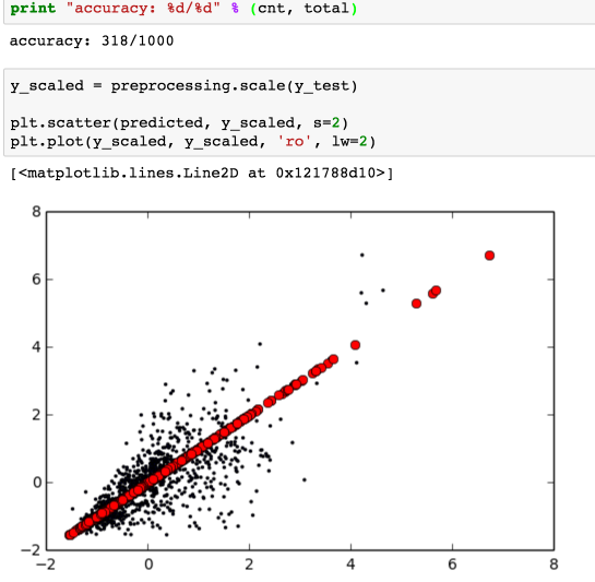
print "accuracy: %d/%d" % (cnt, total)  

输出：

accuracy: 268/1000  

额，不到三成 ...

还有一种优化方案，就是链接2中的 Wider Network Topology，加大第一层的神经元数：

def nn_model():  
    model = Sequential()
    model.add(Dense(20, input_dim=13, kernel_initializer='normal', activation='relu'))
    model.add(Dense(10, kernel_initializer='normal', activation='relu'))
    model.add(Dense(5, kernel_initializer='normal', activation='linear'))
    model.add(Dense(1, kernel_initializer='normal'))
    model.compile(loss='mae', optimizer='rmsprop')
    return model

从结果来看确实有所提高准确度：

最后我们捏造两个数值来比较下 Keras 和 SVR 两种模型：

下面两组数据，一个是在天河区靠近地铁三号线 200 米左右有学位的房子；一个是在花都区没挨着地铁没学位的房子，两组数据其他都一样：

房,厅,卫,建筑面积,建筑年代,朝向,楼层,装修,地铁沿线,地铁距离,区,学校,有无电梯
3.0,2.0,2.0,133.0,7.0,2.0,2.0,4.0,3.0,200.0,1.0,1.0,1.0  
3.0,2.0,2.0,133.0,7.0,2.0,2.0,4.0,0.0,0.0,9.0,1.0,1.0  

结果：

| 房源 | Keras    | SVR      |
| 天河 | 80271.16 | 69902.54 |
| 花都 | 11703.23 | 14411.85 |

都正确地预估出天河的房子要比花都的要贵好多。

就这两组数据来说，个人感觉 Keras 比 SVR 更符合现实 ...

搭个页面应用

最后我们用 Flask 搭个简单的单页应用来做个房源估价应用。

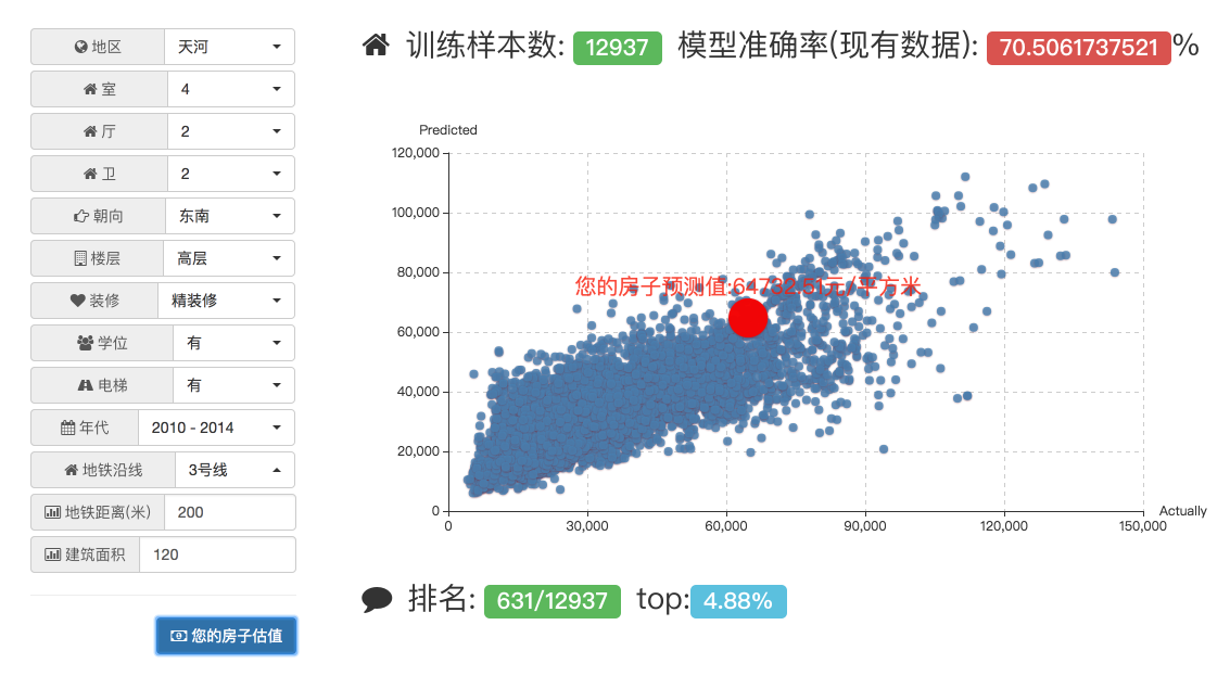
使用的是之前训练出来的 SVR 模型。

结论

• 得益于各种开源项目，目前上手机器学习和深度学习，门槛降低了很多；
• 房价还在疯狂上涨，我去 ...